How Much Can a Zero-Knowledge Proof Leak?

tl;dr Recently, Marshall Ball and I released work on the computational complexity of multiplicative zero-knowledge (MZK), a new definition of zero-knowledge, and its relation to a well-studied definition of zero-knowledge, statistical zero-knowledge (SZK). We show that up to a certain level of leakage, both definitions are equivalent in terms of computational power. That is, allowing (logarithmic) leakage can change how we prove a statement without changing whether the statement belongs to SZK.Then as we allow more leakage, MZK becomes closer in power to IP/PSPACE (i.e., can solve all problems that interactive proof systems can solve). In my class, starting next week, we will begin discussing zero-knowledge definitions and protocols.

Motivations

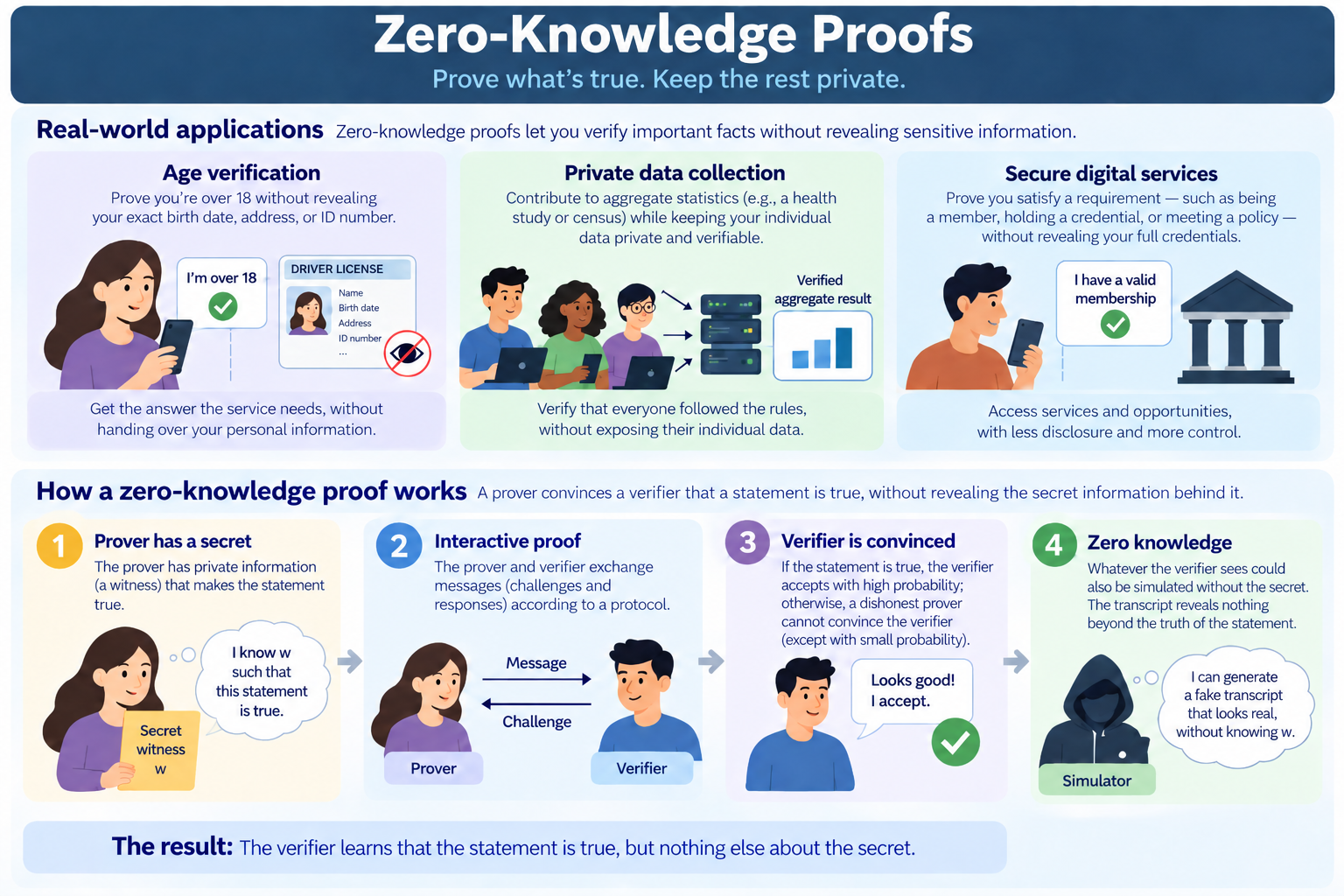
Suppose a website needs to check that you are over eighteen. One approach is to upload a photograph of your identification. But that may reveal much more than the website needs: your exact birth date, address, photograph, and identification number. However, the question the website needs answered is actually much narrower: Does this person satisfy the age requirement?

Zero-knowledge proofs offer a way to separate that answer from the information used to establish it. A person can prove that an authentic credential satisfies an age requirement without handing over the underlying credential. This is a concrete application of the technology: Google’s digital-identity documentation describes zero-knowledge proofs for verifying claims such as “over eighteen” while minimizing disclosure of credential information.

Here is another example: A service might want aggregate statistics without seeing individual contributions. Yet privacy alone is not enough: malicious participants could submit malformed values that corrupt the result. The system needs to verify that contributions satisfy its rules without exposing them. Prio, for example, combines private aggregation with secret-shared proofs that help protect the computation against malicious clients.

These two applications share a common theme:

How can we verify that someone followed the rules without demanding the private information that makes verification easy?

It turns out that zero knowledge is the right tool! And there are several different definitions that imply a surprisingly rich tradeoff between privacy, efficiency, and computational power.

In a recent work, Marshall Ball and I study whether and how multiplicative relaxation of zero-knowledge (MZK) is related to statistical zero-knowledge (SZK). It turns out MZK can improve efficiency, relative to SZK, without enlarging the class of provable problems but when leakage is at most logarithmic. At larger leakage budgets, we show both conditional and oracle separations, and shows that polynomially bounded leakage eventually recovers the full power of interactive proofs.

Our work was driven by the following questions: Can allowing leakage make a proof cheaper? And can allowing leakage make a fundamentally different kind of statement provable?

First, let’s recall the (high-level) definition of zero-knowledge.

What does “zero knowledge” actually mean?

A proof system has a prover, who tries to prove a public statement, and a verifier, who checks it. A useful system must convince the verifier when the statement is true, while preventing a dishonest prover from successfully proving a false statement (except with a small probability). Zero-knowledge adds a privacy requirement: the interaction should not give the verifier information beyond what it could efficiently generate from the public statement itself.

That last requirement is formalized through a simulator: Imagine a program that receives the public statement but not the prover’s secret evidence (called the witness). The simulator must produce an artificially created record of what the verifier would see during the proof. If that record looks like a real interaction, the verifier has not obtained something that required access to the prover’s secret. Note that the simulator is not discovering the secret nor proving the statement through a genuine interaction. It is manufacturing a record. The difference matters: a real cheating prover must answer challenges as they arrive, while an offline simulator can construct a whole conversation in a different order. A simulator transcript need not be something a prover could generate while interacting with an independently randomized verifier.

Essentially, to prove privacy, we will look at two distributions: $R=$ the verifier’s view in a real proof, $Q=$ the simulator’s output.

Different notions of zero-knowledge impose different requirements on how closely these distributions must agree.

Why statistical zero-knowledge?

In statistical zero-knowledge, or SZK, the real and simulated views must have negligible statistical distance. Recall that statistical distance measures the largest difference in probability that the two distributions assign to any event: $SD(R,Q) = \sup_E |R(E)-Q(E)|.$ Here, by “negligible”, we mean that the difference eventually becomes smaller than every inverse polynomial in the security parameter. The privacy requirement is therefore much stronger than saying that the distributions are merely similar on average. This gives statistical zero-knowledge an operational interpretation. Once the real and simulated views are statistically close, even an observer with unlimited computational power cannot distinguish those two distributions with more than negligible advantage. (This holds regardless of whether the observer is able or unable to solve a difficult computational problem.)

For comparison, computational zero-knowledge requires only that efficient observers/adversaries be unable to distinguish the distributions to gain information. The difference is between information that is statistically absent and information that is computationally inaccessible.

There is also an important difference between privacy and soundness. In complexity theory and cryptography, a proof must remain sound against computationally unbounded cheating provers. On the other hand, an argument only needs to hold against computationally bounded cheating provers. For this blog post, we only consider proofs.

SZK is a class of problems: it is about families of statements that admit proof systems with statistical simulation. Our paper follows the standard formulation, in the literature, using promise problems, where inputs are guaranteed to belong to specified yes- or no-cases.

An example: proving that two networks are different

Two graphs are isomorphic when renaming/relabelling their vertices makes them identical. Now consider the problem of proving that two graphs are not isomorphic. The verifier secretly chooses one graph, randomly renames its vertices, and sends the result to the prover. The prover identifies which original graph was chosen. If the graphs are non-isomorphic, a (powerful) prover can always answer correctly. If they are isomorphic, the challenge has the same distribution whichever graph was chosen, so no prover can guess the hidden choice with probability greater than one half.

For an honest verifier, simulation is straightforward: choose the graph and relabeling, then record the already-known answer. This gives perfect honest-verifier zero-knowledge (which is stronger than statistical distance closeness). Note that this simple protocol does not by itself lead to security against arbitrary cheating verifiers; that requires additional machinery.

A second example: proving that distributions are distinguishable

A more general example is Statistical Difference. The input consists of two efficient randomized programs, with a promise that their output distributions are either close or far apart.

Sahai and Vadhan [4] showed that this problem is complete for SZK: every problem in SZK can be (efficiently) converted into the statistical distance problem. Their work also develops transformations that polarize statistical distance, turning a suitable initial gap into distributions that are almost identical or almost disjoint. In the latter case, a prover can help a verifier identify which distribution generated a challenge sample. In our new paper, we leverage such promise problems to show equivalences (up to logarithmic leakage) between SZK and MZK.

Replacing statistical closeness with multiplicative closeness

Statistical zero-knowledge requires probabilities to agree up to a negligible additive difference. Multiplicative zero-knowledge, or MZK, instead permits a (controlled) multiplicative difference:

For every event $E$ , it requires $R(E)\le e^\varepsilon Q(E)+\delta$ and $Q(E)\le e^\varepsilon R(E)+\delta.$

Here, $\varepsilon$ controls multiplicative leakage, while $\delta$ is an additive simulation error. Both directions actually matter for the definition: neither distribution may assign an event substantially more probability than the other permits. When $\delta=0$ , the probabilities of any event (with positive probability) under either distribution differ by at most a factor of $e^\varepsilon$ . (When $\varepsilon=0$ , the two inequalities reduce to the statistical distance guarantee.)

The definition of MZK is, obviously, inspired by differential privacy. But the objects being compared are different. Differential privacy typically compares outputs on neighboring datasets. Here, the comparison is between a real interaction and a simulated interaction. There need not be any neighboring input relation. The relaxation can be substantial even when $\varepsilon$ is constant. For an elementary illustration, suppose $R(1)=\frac34, Q(1)=\frac14.$ These Bernoulli distributions have statistical distance $1/2$ , yet satisfy pure symmetric multiplicative closeness with $\varepsilon=\ln 3$ . Thus, constant multiplicative leakage does not imply negligible statistical leakage. Nor should $\varepsilon$ be read literally as the number of secret bits disclosed. It is a bound on probability/likelihood ratios.

Why relax zero-knowledge at all? Because of savings in communication

A privacy definition is useful partly because of the protocols it enables. Requiring a stronger simulation guarantee can mean sending more information, performing more computation, or using a more expensive interaction pattern.

PINE provides a concrete example. It verifies a norm bound on a secret-shared vector: a useful task when private contributions must be prevented from having excessive influence on an aggregate. Its statistical and differential variants have different communication costs. Under one parameter setting reported in the paper, the additional communication above basic aggregation is:

Vector dimension	Statistical PINE	Differential PINE
10,000	22%	4.77%
100,000	3.18%	1.46%
1,000,000	0.49%	0.32%
10,000,000	0.13%	12.63%

These results use $\varepsilon=0.1$ , with soundness and additive privacy errors set to $2^{-50}$ . They show the side-by-side results: multiplicative simulation can reduce overhead, but it does not improve every parameter regime. We emphasize that these percentages measure overhead, not total-communication reduction factors.

A separation for the same distributed task

In our recent work, we also give a theoretical explanation for the separation in communication costs.

We fix a randomized functionality. Suppose $m$ parties each hold a private bit $x_i$ . They want a common random output whose probability of being one is $\Pr[O=1] = \frac14+\frac{1}{2m}\sum_{i=1}^{m}x_i.$ The goal is not to reveal the individual bits, but to produce this specified (aggregate-dependent) random outcome. For powers of two $m$ , in our work, we construct a protocol using $(m-1)(\log_2 m+2)=O(m\log m)$ bits with constant multiplicative leakage of $\varepsilon=\ln 3$ and negligible additive error. In contrast, statistical simulation with error at most $1/(100m^2)$ requires $\Omega(m^2)$ communication. This is an unconditional separation for the specific setting we consider in the paper (see appendix A): private channels, independent private randomness, no correlated setup, fixed public communication schedule, and passive coalitions containing fewer than one third of the parties.

Note that this distributed setting is different from the single-prover, public-statement setting used to define SZK and MZK as complexity classes. But this motivates our exploration into MZK: Relaxing simulation can save communication even when the task/function being computed remains the same. But does this always change which problems admit proofs? We provide a negative answer!

A surprise: logarithmic leakage in MZK does not enlarge set of SZK problems

For me, this was surprising! Let $n$ denote the input length. One of our main theorems is that, with negligible completeness, soundness, and additive simulation errors, $\boxed{ \mathrm{HVMZK}[\varepsilon] = \mathrm{MZK}[\varepsilon] = \mathrm{SZK} \qquad \text{for }\varepsilon(n)=O(\log n). }$

The honest-verifier class, HVMZK, requires simulation only for the prescribed/honest verifier. MZK requires simulation against every efficient verifier, including verifiers that deviate from the protocol. At logarithmic leakage, both classes coincide with SZK. This is surprising because multiplicative closeness can be much weaker than statistical closeness. (The earlier Bernoulli example already showed that even constant multiplicative leakage permits constant statistical distance.)

How can these facts coexist? Because the theorem is about the existence of proof systems for a problem, not the privacy of a particular transcript distribution. A problem might have a very efficient multiplicative zero-knowledge protocol whose transcripts are not statistically simulatable. The theorem says that the same problem also has some statistical zero-knowledge proof. That is, the statistical zero-knowledge proof may use a different interaction and have different costs. The theorem does not imply that we will preserve the original protocol’s efficiency or statistically simulate its original transcripts.

Why does a logarithm appear?

For some constant $C$ , consider $\varepsilon(n)=C\log n,$ then $e^{\varepsilon(n)}$ is polynomial in $n$ . But when $\varepsilon(n)$ grows faster than logarithmically, that factor becomes superpolynomial. Consider the event $A$ that a simulated conversation is valid and accepting. On a true statement, the real proof accepts with high probability. Then by definition, we get $Q(A) \ge e^{-\varepsilon}\bigl(R(A)-\delta\bigr)$ , where $Q$ is the distribution over the simulator outputs and $R$ is the view of the (real) prover-verifier interaction. At logarithmic leakage, this guarantees at least inverse-polynomial accepting probability. A polynomial-time procedure can therefore repeatedly run the simulator and obtain an accepting conversation with very high probability.

But an accepting conversation might have been assembled using correlations that a real prover could not create. For example, an early answer correlated with a verifier’s (still-hidden) future randomness. So, finding accepting transcripts therefore does not lead to soundness. We addresses this via a causality constraint using a simulation-based prover and relative entropy. On yes-instances, symmetric multiplicative simulation leads to a logarithmic relative-entropy bound (after suitable regularization). On no-instances, an efficiently sampled distribution that accepts often must be much farther, in relative entropy, from the corresponding genuine online prover’s view, because soundness forces that prover to accept only negligibly often. Then an entropy-chain-rule identity translates this gap into instances of Entropy Difference, while Statistical Difference handles insufficient accepting mass. These are both SZK-complete problems, giving the desired reduction.

Beyond logarithmic leakage

In our paper, we give several ways in which larger leakage budgets permit greater computational power. Some are unconditional class characterizations; some require complexity assumptions; others establish separations in oracle settings.

SAT at linear leakage: an (intentionally) revealing protocol

The SAT problem (which we study in CS/ECE 374 at UIUC!) is about whether a Boolean formula has a satisfying assignment. Let the formula have encoding length $n$ and $m\le n$ variables. Fix a satisfying assignment $w$ . Consider the following prover:

With probability $1-2^{-n}$ , send $w$ . With probability $2^{-n}$ , send a uniformly random $m$ -bit assignment.

The verifier checks whether the received assignment satisfies the formula. The simulator simply sends a uniformly random assignment every time. Writing $\eta=2^{-n}$ , the message distributions are $R_w(y) = (1-\eta)\mathbf 1[y=w]+\eta 2^{-m}, Q(y)=2^{-m}.$ At the satisfying assignment, the ratio $R_w(y)/Q(y)$ is at most $2^m\le 2^n$ . Away from it, the reverse ratio is exactly $1/\eta=2^n$. Consequently, both multiplicative inequalities hold with $\varepsilon=n\ln 2, \delta=0.$

The protocol has perfect soundness and completeness error at most $2^{-n}$ . Because the proof consists of one prover message, the same multiplicative bounds extend to an arbitrary efficient verifier’s entire view by randomized post-processing. Thus, $\mathrm{SAT}\in\mathrm{MZK}[n\ln 2,0].$ It is known that, unless the polynomial hierarchy collapses to its second level, SAT does not belong to SZK. This gives a conditional separation between linear-leakage MZK and SZK.

A remark about privacy: This protocol reveals a satisfying assignment with overwhelming probability. It is clearly not private in the ordinary sense one would want for a credential or confidential computation. It satisfies MZK because the allowed multiplicative factor is enormous! The rare random branch does the following: it gives the real distribution positive probability wherever the simulator has positive probability. Without it, the simulator could output assignments that the real prover never sends, making pure symmetric multiplicative simulation impossible.

Polylogarithmic leakage: conditional separations much closer to the boundary

An interesting regime lies between logarithmic and polynomial leakage.

For fixed integers $j\ge1$ , define $\mathcal M_j = \mathrm{MZK}[O((\log n)^j)].$ We show that $\mathrm{SZK}=\mathcal M_1 \subseteq \mathcal M_2 \subseteq \mathcal M_3 \subseteq\cdots.$ That is, for every $\mathcal M_j$ with $j\ge2$ strictly contains SZK under a specific nonuniform circuit hardness assumption: some fixed-width DNF tautology problem has no subexponential-size nondeterministic circuits. This assumption follows from a nonuniform nondeterministic version of the Strong Exponential Time Hypothesis.

Two things to note: (i) the argument does not use ordinary uniform SETH, and (ii) the result separates each higher level from SZK; it does not prove that successive levels differ from one another.

Oracle separations in a black-box setting

We prove a separation for every polynomial-time computable, polynomially bounded superlogarithmic integer profile $\ell(n)$ . For each such profile, there is an oracle $A$ and a language that belongs to $\mathrm{MZK}^{A}[(\ell(n)-1)\ln 2,0]$ but not even to quantum statistical zero-knowledge relative to that oracle. This covers profiles as close to logarithmic as $\log n\log\log n$ , as well as $(\log n)^2$ . An oracle is an idealized black box available to the algorithms under comparison. Such a separation is not an unconditional separation of the ordinary classes. The implication here is that the equality of SZK to MZK, under logarithmic leakage, cannot be extended to all larger budgets.

The appearance of quantum SZK strengthens the oracle result: even allowing quantum statistical-zero-knowledge (larger than SZK) protocols does not eliminate the separation in the constructed setting.

At polynomial leakage, MZK recovers all interactive proofs

Another result is that $\boxed{ \mathrm{MZK}[\mathrm{poly}] = \mathrm{HVMZK}[\mathrm{poly}] = \mathrm{PSPACE}. }$

Here, “poly” means the union over polynomial leakage bounds. The equality holds even with zero additive simulation error. PSPACE consists of problems solvable using polynomially bounded memory, potentially with much greater running time! A result of Shamir shows that $\mathrm{IP}=\mathrm{PSPACE}$ ; so PSPACE consists of exactly the problems admitting polynomial-time verifier interactive proofs. Our result, therefore, implies that sufficiently large multiplicative leakage removes the language class restriction imposed by statistical zero-knowledge. The construction, for this result, generalizes the SAT example. Take an interactive proof and modify its prover: almost always follow the original strategy, but on a negligible-probability branch send uniformly random replies. The simulator always uses uniform replies.

If the prover sends at most $b(n)$ bits and the rare branch has probability $2^{-h(n)}$ , the resulting leakage is bounded by $\varepsilon(n) = \ln 2\cdot\max\{b(n),h(n)\}.$ Choosing polynomially bounded parameters with negligible branch probability preserves negligible completeness error and leaves soundness unchanged. Once again, this is a characterization of computational power. Do not use polynomial leakage for actual applications.

What remains open?

How sharp is the separation without oracles or computational (nonuniform SETH) assumptions?

Can one prove an unconditional, unrelativized separation at polylogarithmic leakage? Can the conditional results be obtained from weaker or more familiar assumptions? And what is the right characterization of intermediate profiles such as $\log n\log\log n$ in the ordinary, non-oracle setting?

Is there a strict hierarchy of leakage levels?

In our paper, we give an increasing sequence $\mathrm{SZK}=\mathcal M_1 \subseteq\mathcal M_2 \subseteq\mathcal M_3 \subseteq\cdots,$ but we do not give a result for whether each successive inclusion is strict. Perhaps additional leakage repeatedly increases computational power. Perhaps several intermediate levels coincide.

Can intermediate MZK have a natural complete problem?

In my opinion, SZK benefits enormously from Statistical Difference: a complete problem stated simply in terms of two efficiently samplable distributions. Can a similarly clean problem characterize intermediate-leakage MZK?

What are the best efficiency gains within the SZK regime?

For a given task, how much communication can constant or logarithmic multiplicative leakage save? Which savings survive arbitrary redesign of the statistical protocol? Can a conversion to SZK preserve useful bounds on total communication, rounds, or prover computation?

The distributed separation shows that communication savings can be fundamental in an appropriately specific model. Our logarithmic collapse result shows that those savings need not lead to an enlargement of the corresponding public-input proof class. Essentially, can we turn our complexity-theoretic results into useful protocol-design guidance?

References

[1] Shafi Goldwasser, Silvio Micali, and Charles Rackoff. The knowledge complexity of interactive
proof systems. SIAM Journal on Computing, 18(1):186–208, 1989.

[2] Oded Goldreich, Silvio Micali, and Avi Wigderson. How to prove all NP statements in
zero-knowledge and a methodology of cryptographic protocol design (extended abstract). CRYPTO’ 86.

[3] Oded Goldreich, Silvio Micali, and Avi Wigderson. Proofs that yield nothing but their validity
or all languages in np have zero-knowledge proof systems. J. ACM, 38(3):690–728, July 1991.

[4] Amit Sahai and Salil P. Vadhan. A complete problem for statistical zero knowledge. Journal
of the ACM, 50(2):196–249, March 2003.

[5] Daniel Alabi, Marshall Ball. On the Complexity of Statistical and Multiplicative Zero-Knowledge. Cryptology {ePrint} Archive, Paper 2026/2104. https://eprint.iacr.org/2026/2104

What Does a Diffusion Model Remember?

tl;dr My graduate student (Tue Do) has developed DIME, an efficient membership test based on the theory of the exact optimal denoiser for diffusion models. DIME gives some impressive results: across a range of datasets, DIME consistently outperforms prior attacks at comparable or substantially lower query cost, improving certain metrics by up to 3×; remarkably, its two-query variant can outperform existing 30-query baselines. Check it out!

Diffusion models have become one of the dominant approaches to generative modeling because they can produce remarkably high-quality outputs while remaining relatively stable to train. They underpin many modern image generation and editing systems (e.g., Stable Diffusion, Midjourney, DALL-E, etc.), and related diffusion techniques have also been applied to video, audio, scientific data, inverse problems, and other modalities. Their success comes from a simple but powerful training objective: a model learns to reverse a gradual noising process, transforming corrupted data back toward samples that resemble the training distribution. This denoising formulation scales well to high-dimensional data and gives practitioners considerable control over generation, including conditioning on text, class labels, or other signals.

The widespread use of diffusion models also makes it important to understand what they learn about their training data, not just how good their generated samples look. State-of-the-art models are often trained on enormous collections of images gathered from the web or from sensitive domains such as medicine, biometrics, and personal photography. A model that behaves well at generation may nevertheless retain information about particular training examples. This raises questions about privacy, memorization, copyright, data provenance, and whether a person’s data has actually been removed after a deletion or machine-unlearning request. Membership inference, the problem of determining whether a particular record was used during training, is therefore a useful way to probe the boundary between learning general statistical structure and retaining example-specific information.

Diffusion models are especially interesting from a privacy perspective because their core denoising task is closely related to reconstruction. Given a corrupted input, the model repeatedly estimates information needed to move that input back toward likely clean data. If the model has learned unusually detailed information about a particular training example, its denoising behavior near that example may differ from its behavior near unseen data. Studying these differences helps us understand where memorization lives inside a diffusion model and how it can be detected. This is valuable both offensively, for developing stronger privacy audits, and defensively, for evaluating whether techniques such as differential privacy, deduplication, or regularization actually prevent training examples from leaving detectable traces.

There’s the diffusion model training question: Given a noisy version of an image, what noise was added, or equivalently, what clean image should the model reconstruct? And the membership inference question: Given a candidate image, was this image part of the model’s training set?

In DIME, we exploit the fact that these two questions are, in fact, tightly connected. A perfectly trained diffusion denoiser does not merely learn a generic rule for “what noise looks like.” On a finite training set, its optimal prediction can be written exactly as a posterior-weighted combination of the training examples. The model is therefore carrying out a kind of soft retrieval: given a noisy input, it asks which training points could plausibly have generated it and blends those points according to their posterior responsibilities.

That observation turns membership inference from a search for ad hoc statistics into a derivation. The model’s implicit reconstruction of a candidate has an exact squared error, and that error splits into two terms:

Reconstruction bias: how far the local posterior mean is from the candidate; and
Local crowding: how dispersed the plausible training points are around that mean.

The first signal resembles what earlier norm and reconstruction-based attacks measure. The second is the new ingredient: a non-member can be reconstructed surprisingly well simply because it lies near the center of several training points. Bias alone can therefore be fooled by local geometry, while crowding exposes the ambiguity.

Both signals can be estimated from forward queries to the denoising network. They share the same randomly perturbed queries, so the attack needs only a few model evaluations and its cheapest setting uses just two total queries. In experiments on CIFAR-10, CIFAR-100, STL10-U, CelebA, and ImageNet, DIME improves the low-false-positive detection rate substantially, sometimes beating 30-query baselines with only two queries. We also test the attack against differentially private mechanisms and finds that differentially private training drives DIME and the evaluated baselines back toward chance.

A minimal diffusion refresher

Let the finite training set be

$\displaystyle \mathcal D_{\mathrm{train}}=\{x_1,\ldots,x_n\}\subseteq\mathbb R^d.$

At timestep $t$ , the forward process forms

$\displaystyle g=\sqrt{\bar\alpha_t}\,x+\sigma_t z, \qquad z\sim\mathcal N(0,I_d), \qquad \sigma_t=\sqrt{1-\bar\alpha_t}.$

The noise-prediction network is trained by mean squared error:

$\displaystyle \mathcal L_t(\theta) = \mathbb E_{x\leftarrow\mathcal D_{\mathrm{train}},\,z\sim\mathcal N(0,I_d)} \left[ \left\| \widehat\varepsilon_\theta(\sqrt{\bar\alpha_t}x+\sigma_tz,t)-z \right\|_2^2 \right].$

For squared loss, the population-optimal prediction is a conditional expectation. Here, because the data distribution is the empirical distribution over a finite training set, that conditional expectation can be calculated explicitly.

The first main result: the exact finite-set optimal denoiser

For a query $g$ , define the unnormalized compatibility of training point $x_i$ by

$\displaystyle s_i(g) = \exp\!\left( -\frac{\|g-\sqrt{\bar\alpha_t}x_i\|_2^2}{2\sigma_t^2} \right),$

and normalize these scores into responsibilities

$\displaystyle r_i(g)=\frac{s_i(g)}{\sum_{j=1}^n s_j(g)}.$

We prove that the MSE-optimal denoiser is

$\displaystyle \boxed{ \widehat\varepsilon^*(g,t) = \frac{g}{\sigma_t} - \frac{\sqrt{\bar\alpha_t}}{\sigma_t} \sum_{i=1}^n r_i(g)x_i. }$

This formula has a simple Bayesian derivation. If training point $x_i$ generated $g$ , the corresponding noise would be

$\displaystyle z_i=\frac{g-\sqrt{\bar\alpha_t}x_i}{\sigma_t}.$

Conditioned on seeing $g$ , the posterior probability that the latent training index was $i$ is precisely $r_i(g)$ . The optimal squared-loss estimate is therefore

$\displaystyle \mathbb E[z\mid g] = \sum_i r_i(g)z_i,$

which expands to the boxed expression.

The denoiser is a soft decoder over the training set

The weighted point

$\displaystyle m(g)=\sum_i r_i(g)x_i$

is the model’s implicit reconstruction of the clean training example that could have produced $g$ . Training examples close to $g/\sqrt{\bar\alpha_t}$ receive exponentially larger responsibility. The noise scale $\sigma_t$ acts like a temperature:

at high noise, many records can plausibly explain the query, so responsibilities are diffuse;
at low noise, the posterior sharpens around the closest training record.

As $\sigma_t\to0$ , the soft responsibilities converge almost everywhere to the indicator of the nearest training point’s Voronoi cell. In other words, the ideal denoiser approaches a hard nearest-neighbor decoder.

This explains why membership leakage is strongest in the low-noise regime. For a member $x^*=x_i$ , the nearest point is the record itself, so the posterior can concentrate on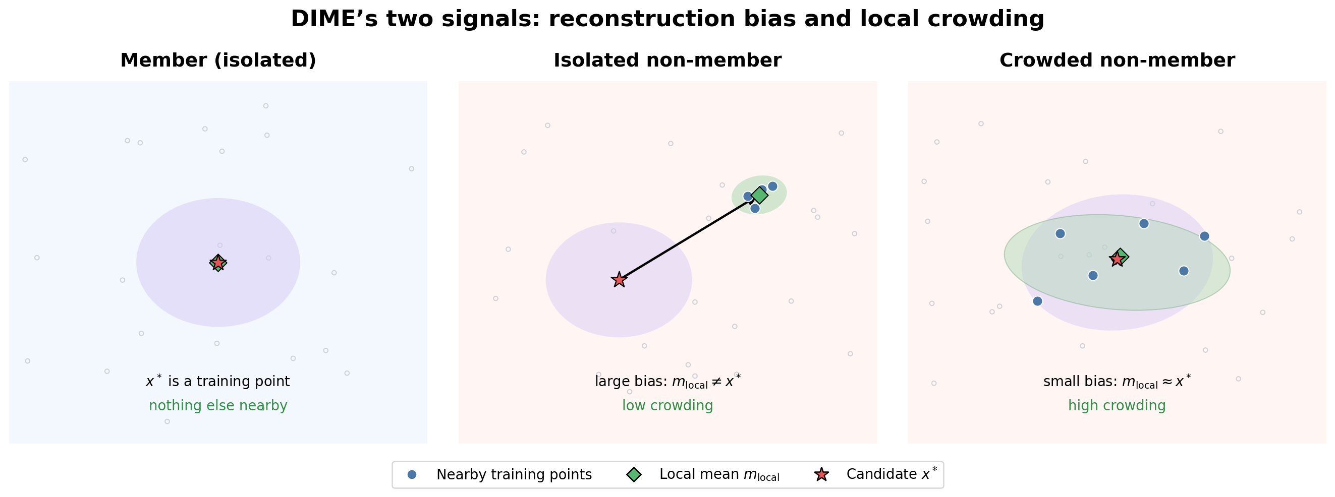 $x_i$ . For a non-member, the best the empirical model can do is retrieve or blend nearby training points.

Why reconstruction bias alone is not enough

The obvious attack would compare the model’s implicit reconstruction with the candidate. A member should reconstruct accurately; a non-member should not. This intuition is useful but incomplete.

A non-member can have small reconstruction bias when it lies near the mean of several training points; the dispersion of those points (the crowding term) distinguishes it from an isolated member.

We separate three cases.

Case A: isolated member

The candidate is itself a training point and has no close competitors. Responsibility concentrates on the candidate. The posterior mean is close to $x^*$ , and the responsible neighborhood has almost no spread. Both bias and crowding are small.

Case B: isolated non-member

The closest training point or cluster lies away from the candidate. The posterior mean is displaced from $x^*$ . Bias is large, even if the nearby training points are tightly grouped.

Case C: crowded non-member

The candidate lies near the center of several training points. Their weighted mean can accidentally be close to $x^*$ , producing small bias. But responsibility is divided among separated records, so the local variance is large.

The one-dimensional example $\mathcal D=\{-1,+1\}$ and $x^*=0$ makes the blind spot exact. If the two records have equal responsibility, the posterior mean is zero, so reconstruction bias is zero even though zero is not in the training set. The variance is one, correctly signaling ambiguity.

What the score distributions and timestep plots show

DIME score distributions from the paper.

Member and held-out DIME score distributions are visibly separated across the five checkpoints; dashed lines show calibrated thresholds.

The distribution plots make the aggregate metrics easier to interpret. DIME is not succeeding because of a handful of extreme outliers; the member and non-member score distributions shift relative to one another across every tested checkpoint. The amount of overlap explains why STL10-U permits near-total detection while CelebA remains harder.

The four smaller DDPM checkpoints remain effective across a broad timestep range, whereas ImageNet Guided Diffusion is most vulnerable at early timesteps.

The ideal denoiser theory predicts stronger concentration at lower noise. Guided Diffusion follows that prediction clearly: attack performance is highest at early timesteps and declines as noise increases. The smaller DDPM checkpoints exhibit a broad plateau instead. This suggests that the roughly 550M-parameter Guided Diffusion model may approximate the ideal denoiser more faithfully than the roughly 35M-parameter DDPM models. This is a plausible interpretation of the observed scale difference, not a formal proof that parameter count is the cause.

An additional practical lesson is that exact timestep selection may not be fragile for the smaller checkpoints. A broad plateau gives an attacker or auditor some tolerance to imperfect calibration.

Synthetic experiments isolate the role of crowding

The real-network experiments inevitably mix two phenomena:

properties of the exact finite-set optimal denoiser; and
approximation and optimization behavior of the trained neural network.

The synthetic appendix removes the second factor by evaluating the closed-form denoiser directly on small, known training sets.

Synthetic bias and variance decomposition from the paper.

The crowded non-member can have relatively small bias, but its variance rises much earlier and separates it from the member.

The left panel shows why a bias-only attack can fail: the crowded non-member’s posterior mean can remain close to the candidate. The middle panel shows the missing signal: responsibility spread creates a nonzero variance well before the member’s variance grows. Their sum in the right panel recovers the intended reconstruction error.

Further synthetic experiments compare DIME with SimA-MC while varying dataset size, noise level, and query count. They show that the extra crowding signal makes DIME’s membership performance decay more slowly as noise increases. These experiments are diagnostic rather than a substitute for the neural-network results, but they confirm that the claimed effect exists in the exact theoretical object itself.

Conclusion

DIME’s central insight can be stated as follows:

A finite-set diffusion denoiser implicitly performs soft retrieval over its training examples, and the error of that retrieval contains both a reconstruction signal and a geometric crowding signal.

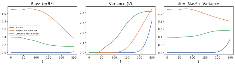
We turn this insight into an exact formula, decompose the corresponding error, link hidden local covariance to the denoiser’s Jacobian, and estimate both terms with $q+1$ forward queries. The resulting attack is not merely more accurate in aggregate; its largest gains occur at the low-false-positive operating point that matters most for credible membership decisions. It also survives a dramatic jump from small unconditional DDPMs to a large class-conditional ImageNet model.

Moreover, the defenses we apply are reassuring: differential privacy suppresses not only earlier heuristic attacks but also the stronger signal produced by the ideal denoiser derivation. The broader message is therefore balanced: Diffusion models can leak membership through richer local geometry than prior attacks measured, but formal stability remains a meaningful line of defense.

DIME provides both a practical attack and a new lens for future work: privacy leakage in diffusion models can be studied as the geometry of a soft decoder over a finite codebook.

References

Tue Do and Daniel Alabi, “DIME: Query-Efficient Framework for Membership Inference on Diffusion Models”, arXiv:2608.22824, 2026.

From Proof Scarcity to Proof Abundance

tl;dr anyone who previously used or currently uses mathematical tools to solve problems in their field (whether in sciences, pure or applied mathematics, engineering, economics, and so on) needs to pay attention to discussions around the use of AI to solve mathematically precise problems. The revolution has begun!

Here’s what I believe: once AI-assisted proofs become abundant, their scarcity value will fall and attention will shift toward the harder tasks of formulating compelling conjectures, building theories, and creating definitions that organize rapidly expanding bodies of results. The analogy is economic: just as an influx of currency can produce inflation rather than lasting wealth, an influx of proofs can reduce the value attached to any individual proof without necessarily producing a comparable increase in understanding.

Firsthand Experience

Honestly, for me, the question of how useful AI could be in solving math problems did not begin in 2026. In November of 2022, ChatGPT was released. I had just begun my postdoc. With support from the Simons Foundation, I started thinking seriously in 2022 about what mathematics (and intellectual work more broadly) might look like in a world with advanced AI. At the time, much of this remained speculative: What would happen if mathematical reasoning became inexpensive? Which parts of research would retain their value? Would the bottleneck shift from proving statements to identifying the right questions, definitions, and conceptual frameworks?

At ICM (International Congress of Mathematicians) 2026, Terence Tao gave a lecture on Mathematics in the Age of AI. I’d encourage everyone to, at least, read the slides! Tao disusses the implications of the abundance of proofs (not necessarily correct). Recent events have made this transition feel concrete rather than hypothetical. While I was watching the 2026 World Cup final, Levent Alpöge announced a counterexample (credited to the AI system Fable) to the Jacobian conjecture. More precisely, the construction disproves the conjecture in dimension three, and therefore in every dimension $n\geq 3$ , while the two-dimensional case remains open. The counterexample has a nonzero constant Jacobian determinant but maps three distinct points to the same output, directly contradicting the conjectured invertibility.

In recent days have also tested advanced AI systems on several problems from my own active research agenda. These were not merely exercises with known answers: in multiple cases, the systems made progress that appeared genuinely novel, uncovering arguments or directions that I had not previously considered. The important question is no longer whether AI can occasionally imitate mathematical reasoning. It is now clear that AI can perform at least some research-level mathematics. The remaining questions concern the breadth and reliability of that ability, the amount of human guidance and computation it requires, and, most importantly, how the mathematical community should evaluate, explain, verify, and build upon the resulting work.

Terence Tao on Mathematics in the Age of AI

In the rest of this blog post, I will highlight a few parts of his talk which I found illuminating!

Tao identifies the central challenge posed by mathematical AI: not merely generating correct proofs, but transforming those proofs into shared human understanding. That is, the most important question is no longer whether artificial intelligence can prove difficult theorems. I believe that Tao deliberately set that question aside. Instead, he asked what may be a more consequential question:

If AI systems become capable of performing a substantial fraction of research-level mathematical work, what exactly should the mathematical community be trying to accomplish?

We all need to think of that shift (from technological capability to institutional purpose). Most discussions of AI and mathematics focus on benchmark performance: Can a model solve Olympiad problems? Can it formalize a proof in Lean? Can it make progress on an open conjecture? Tao’s lecture asks what happens after the answer to some of those questions becomes yes. Tao asks the audience to provisionally assume that reasonably capable mathematical AI is coming. He then investigates what follows for proof, exposition, reviewing, education, authorship, and the organization of mathematical knowledge.

What I appreciate from the talk is that the resulting picture is neither utopian nor apocalyptic. (Although a large fraction of folks see it as a warning.) Clearly, we are headed towards an era in which proofs are scarce to one in which proofs are abundant; our present institutions are designed almost entirely for the former world, where proofs are not abundant.

A crisis of values rather than a crisis of logic

In the late nineteenth and early twentieth centuries, mathematicians were forced to examine assumptions that had previously remained largely implicit. Russell’s paradox, the emergence of competing foundational programs, and Gödel’s incompleteness theorems created a period of uncertainty about sets, numbers, infinity, axioms, and formal proof. This led to the development of more explicit and standardized foundations that gave mathematicians a trusted environment in which to work.

Tao suggests that AI is producing a comparable period of turbulence, although the foundations now at issue are not primarily logical. They are the foundations of mathematical values and practices: what counts as progress, who deserves credit, what authors are responsible for, why proofs matter, and what the profession is ultimately trying to produce. A disruptive development can expose assumptions that were previously invisible because they rarely came into conflict. Before AI, several goals of mathematics tended to advance together. A mathematician who solved a difficult problem often developed a new technique, trained students, wrote an influential paper, helped organize a research community, and contributed to a larger theory. Because those outputs were correlated, institutions could reward one visible quantity, such as the publication of a paper with one or more important theorems, and assume that the others would follow.

AI threatens to break those correlations.

The two questions that are often confused

Tao separates the AI debate into two questions.

The first is a capability question: Will AI tools, at an acceptable cost and with some level of human supervision, be able to perform meaningful research-level mathematical tasks with a nontrivial rate of success?

Tao formulates this as a family of conjectures because almost every term requires qualification. Which tools? Which fields? What counts as research-level? How much supervision? At what cost? What success rate? What standard of correctness? What standard of exposition? A system that autonomously proves 80 percent of new theorems in algebraic geometry is very different from one that occasionally completes a technical lemma after several days of expert prompting. Both might satisfy some version of an AI capability claim. Tao also stresses that public evidence is affected by reporting bias, commercial incentives, undisclosed compute budgets, selective demonstrations, and ambiguous levels of human assistance. The truth of a capability claim must also be separated from whether that capability is desirable.

The second question is a question about goals and values: What are the mathematical community’s actual objectives, including the implicit objectives encoded in publication, hiring, funding, prizes, and professional prestige? Tao’s key methodological move is to condition on a working hypothesis: suppose that a reasonably strong version of the capability claim becomes true reasonably soon. He does not ask the audience to endorse or welcome the hypothesis. He asks what the community should do if it holds. Very reasonable! This is a useful form of reasoning under uncertainty. To continue to do mathematics, we cannot wait until every capability forecast is resolved before examining whether our institutions are robust to rapid automation. Even a moderate probability of large changes can justify preparing publishing policies, authorship standards, review infrastructure, and educational norms.

First Proof

Tao briefly points to the First Proof project as one of the better-controlled pieces of evidence about current AI capabilities. For its second batch, First Proof assembled ten unpublished research-level problems originating in the work of research mathematicians. Four systems were tested in a controlled environment. The outputs were evaluated using a double-blind journal-review model involving approximately thirty experts, with each submission examined by multiple referees. Across the four systems, seven of the ten problems received at least one solution judged essentially correct or in need of only minor revisions. One system found a novel solution to a stochastic partial differential equations problem that differed from the human proof and impressed the referees. Other problems saw little or no meaningful progress.

The results are substantial, but their limitations are equally informative. The systems often handled routine portions of an argument in meticulous detail while moving too quickly through the genuinely difficult step. Referees found unsupported appeals to supposedly standard arguments, incorrect or missing citations, unnecessary notation, and lengthy explanations of facts that an expert would normally omit. Some submissions reproduced distinctive language and notation from earlier work without appropriate attribution (i.e., behavior that would raise serious plagiarism concerns in a human submission).

The computational costs also varied dramatically. In the reported runs, per-problem costs ranged from single-digit dollar amounts to nearly one thousand dollars, depending on the system and problem. This reinforces Tao’s point that “AI solved the problem” is not a complete scientific statement without information about models, harnesses, prompts, search procedures, human intervention, tokens, time, and cost.

Most importantly, First Proof evaluated only one part of mathematical research: generating proofs of questions selected and formulated by humans. Its organizers explicitly distinguish solving questions within existing frameworks from the equally important work of asking new questions and developing the frameworks in which those questions become meaningful.

Mathematics has more than one objective

What is mathematical research for?

Tao identifies several answers:

solving pure and applied problems;
building theories and techniques;
understanding the natural and social world;
training future mathematicians (part of my job);
sustaining a mathematical community;
contributing to a shared network of knowledge;
creating works of enduring intellectual or aesthetic value.

Historically, progress along these dimensions was positively correlated. Solving an important problem often required theory building. Theory building produced reusable techniques. Writing and teaching those techniques helped train students and build a community. This made it tempting to treat theorem production as a proxy for mathematical progress. Tao invokes Goodhart’s law: once a proxy becomes an explicit target, optimization can destroy the relationship that made the proxy useful. AI makes this danger especially severe because it can lower the cost of producing objects that look like the outputs rewarded by current metrics.

Suppose an institution rewards:

the number of problems solved;
the number of papers published;
being first to announce a proof;
benchmark scores;
citation counts;
the number of formalized theorems.

An AI-intensive workflow may increase each of these without proportionately increasing understanding, theory, pedagogy, reliability, or long-term usefulness.

A thousand isolated proofs are not necessarily more valuable than one conceptual framework explaining why all thousand theorems are true. A technically correct argument is not necessarily a useful argument. A formally verified statement is not necessarily the statement that mathematicians intended to prove. A highly cited result is not necessarily well understood.

The deeper point is that mathematical knowledge is not a warehouse of theorem statements. It is an organized system of concepts, explanations, analogies, techniques, examples, counterexamples, and judgments about what matters.

Tao’s proposed “oral defense” standard

Tao offers a rule of thumb: a result should not be published unless its human authors can convincingly present a clear, correct, properly attributed expert-level explanation of it. The proposal addresses several problems simultaneously.

An author capable of defending the result is more likely to have:

checked that the theorem says what it is supposed to say;
located the crucial step;
understood the relationship to prior work;
detected misleading AI-generated exposition;
assumed meaningful responsibility for correctness.

The idea resembles a thesis defense. Producing a document is not enough; the author must demonstrate command of its content. As a literal universal publication requirement, however, the rule would need careful implementation. It is bound to be controversial: Oral presentation ability varies, and a rigid talk requirement could disadvantage researchers with disabilities, non-native speakers, or authors whose strengths lie in writing rather than performance. Large collaborations may also have genuinely distributed understanding.

The underlying principle is stronger than any particular format: publication should require evidence of human intellectual ownership and accountability. That evidence might take the form of a seminar, an annotated proof map, a technical interview, an expository companion, or an independent human audit. (I’m hoping to implement the oral defense standard within my research group.)

Selected references and further reading

Terence Tao, Mathematics in the Age of AI, ICM public-lecture slides, July 24, 2026. (Teorth)

Mohammed Abouzaid et al., First Proof: Second Batch Report, 2026. (First Proof Project)

William P. Thurston, On Proof and Progress in Mathematics, Bulletin of the American Mathematical Society, 1994. (arXiv)

Tanya Klowden and Terence Tao, Mathematical Methods and Human Thought in the Age of AI, 2026. (arXiv)

Johan Commelin, Mateja Jamnik, Rodrigo Ochigame, Lenny Taelman, and Akshay Venkatesh, Shaping the Future of Mathematics in the Age of AI, 2026. (arXiv)

Jeremy Avigad, Mathematicians in the Age of AI, 2026. (arXiv)

Leiden Declaration on Artificial Intelligence and Mathematics, June 2026. (Leiden AI & Math Declaration)